Code for this blog post can be found at link

I recently read this paper on Hamiltonian Neural Networks, and thought it was pretty neat.

The idea is this: Is there a way that we can teach neural networks basic laws of physics? One might say that given sufficient data, the network should learn the underlying physical law, but it turns out that to do this you need quite a lot of data, and you still don’t have a formal guarantee that the network is learning the true physics.

Hamiltonian neural networks are a simple method of enforcing physical constraints on the neural network. To understand how and why they work, we need to talk about Hamiltonian mechanics.

Hamiltonian Mechanics

Newton’s Laws: Forces & Second-Order ODEs

Hamiltonian mechanics is an alternative formulation of classical mechanics to Newton’s laws. In Newtonian mechanics, you start with in order to determine the so-called equation of motion of an object, we apply Newton’s second law: $$\vec{F} = m\vec{a}$$. That is, we take our object, determine what the forces on it are, and then that tells us the acceleration of the object, from which we can calculate its position over time via some second order differential equation.

Pendulum in Newtonian Terms

• Coordinate: angle \(\theta\).
• Force: The tangential component of gravity $$ F_\theta = -mg\sin\theta.$$
• Equation of motion:
  $$ mL\,\ddot\theta = -mg\sin\theta\quad\Longrightarrow\quad\ddot\theta + \frac{g}{L}\,\sin\theta = 0.$$

This equation can then be solved numerically.

Hamiltonian Mechanics: Energy & First-Order Flow

In Hamiltonian mechanics, we don’t consider forces. Instead, we consider a scalar function of the coordinates, call the Hamiltonian, \( \mathcal{H}(q, p, t),\) usually the total energy (kinetic + potential), expressed in terms of:

• \(q\): generalized coordinate (e.g. $(\theta)$ for the pendulum)
• \(p\): conjugate momentum (for a pendulum, \(p = mL^2\,\dot\theta\))
• \(t\): sometimes explicitly, if energy isn’t conserved

Then the equations of motion are a neat pair of first-order ODEs:

\(\dot q = \frac{\partial \mathcal{H}}{\partial p}, \quad \dot p = -\,\frac{\partial \mathcal{H}}{\partial q}.\\)

The Simple Pendulum in Hamiltonian Mechanics

1. We can start by writing the Hamiltonian, $$\mathcal{H}(\theta,p) = \frac{p^2}{2\,m\,L^2} + mgL(1-\cos\theta).$$
2. Putting that into Hamilton’s equations, we get
   • $ \dot\theta = \frac{\partial \mathcal{H}}{\partial p} = \frac{p}{mL^2} $
   • $ \dot p = -\frac{\partial \mathcal{H}}{\partial \theta} = -mgL\sin\theta $
3. Simulate these two first-order equations (often with a symplectic integrator like Verlet) and you’ll see the same nice, closed loops in \((\theta,p)\)-space.

Connection to Lagrangian mechanics

If you’ve done Lagrangian mechanics, you know it starts from another scalar function, the Lagrangian
$$ L(q,\dot q) = T(\dot q) - V(q),$$ One then applies the Euler–Lagrange equation:
$$ \frac{d}{dt}\Bigl(\frac{\partial L}{\partial\dot q}\Bigr) - \frac{\partial L}{\partial q} = 0.$$

In order to get to the Hamiltonian picture, we define the conjugate momentum
$$ p = \frac{\partial L}{\partial \dot q},$$ and then the Hamiltonian is just the Legendre transform:
$$ H(q,p) = p\,\dot q - L(q,\dot q).$$

Neural Simulation

Okay, so how might we train a neural network to simulate our pendulum. In the Hamiltonian formalism, all we need is some way to compute \(\frac{\partial \mathcal{H}}{\partial \theta}\) and \(\frac{\partial \mathcal{H}}{\partial p_\theta}\). Then, we could feed those derivatives into our differential equation solver, and get out some sensible output.

So, naively, we could train a neural network to do predict those derivatives given \(\theta\) and \(p_\theta\). The results are plotted below.

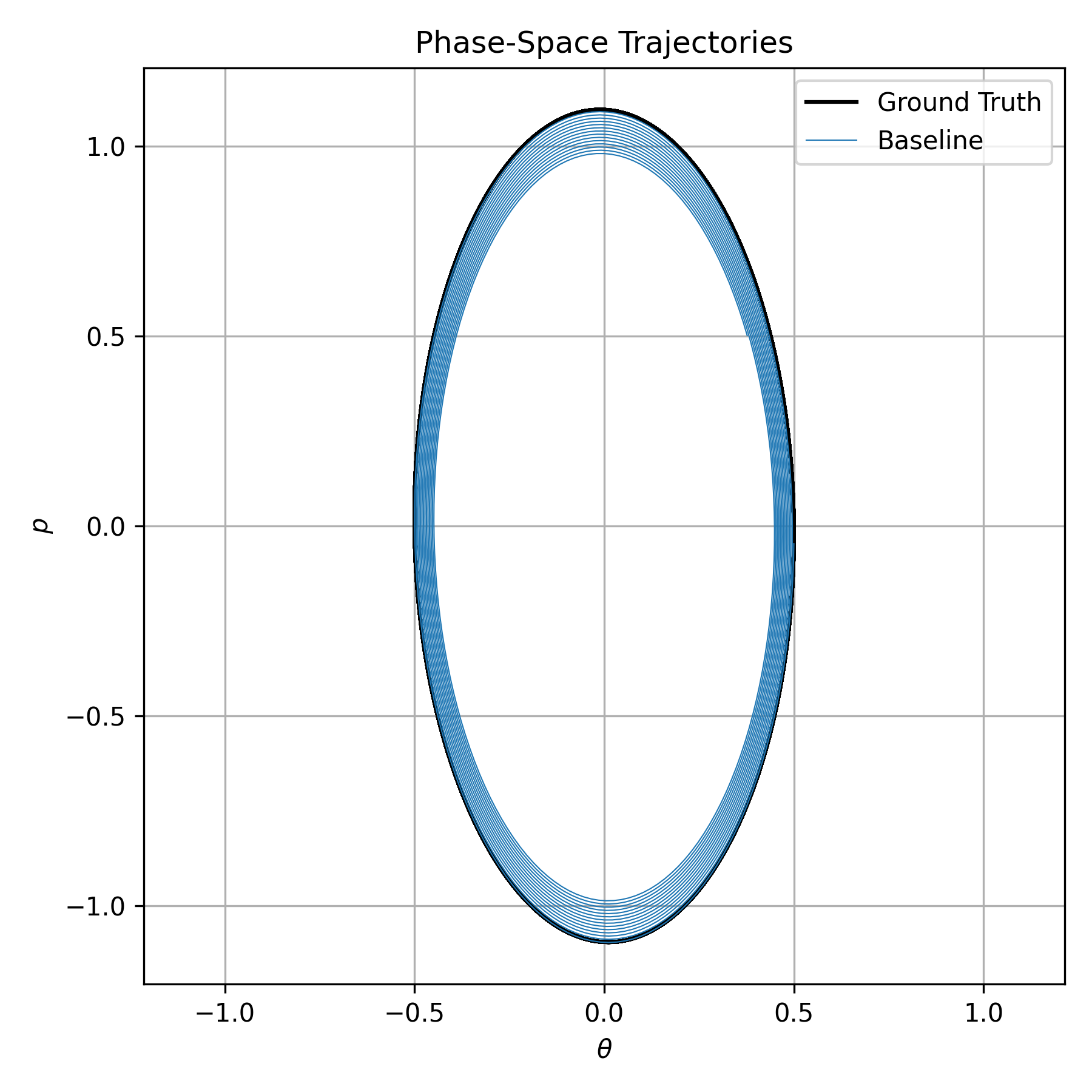
As you can see from the phase space diagram, the ground truth is that the pendulum follows an ellipse in phase space, but the network fails to capture that. The fact that we have a closed loop in phase space demonstrates that our pendulum follows some sort of periodic motion. The fact that our network’s output slowly spirals corresponds to the pendulum slowly losing energy. Why?

1. The Approach
   • We took our \((\theta,p)\) pairs and trained an MLP to output \(\widehat{\dot\theta}\) and \(\widehat{\dot p}\) directly.
   • Loss = mean-squared error between \((\widehat{\dot\theta},\widehat{\dot p})\) and the true changes in angle/momentum, from Hamilton’s equations.
2. Why it fails to close
   • Because nothing in the network knows about energy conservation or symplectic structure, tiny errors in \(\widehat{\dot\theta}\) and \(\widehat{\dot p}\) accumulate over time.
   • When you integrate those “raw” predictions—even with a symplectic integrator—the error in energy creeps in and the orbit slowly spirals in.

Hamiltonian Neural Networks

Hamiltonian neural networks solve this problem by parameterizing the Hamiltonian instead. That is, the neural network takes in the phase space coordinates, and the spits out the Hamiltonian. Then, in order to compute the necessary derivatives for Hamilton’s equations, we just have to backpropagate through the network and compute the gradients of the output with respect to the input!

The network is trained to minimize the error between those backpropagated gradients, and the true time derivatives. It’s a simple, and beautiful idea. We needed to compute those derivatives anyway for gradient descent; by optimizing them, we implictly train the network to satisfy Hamilton’s equations. You can see the results in the figure below.

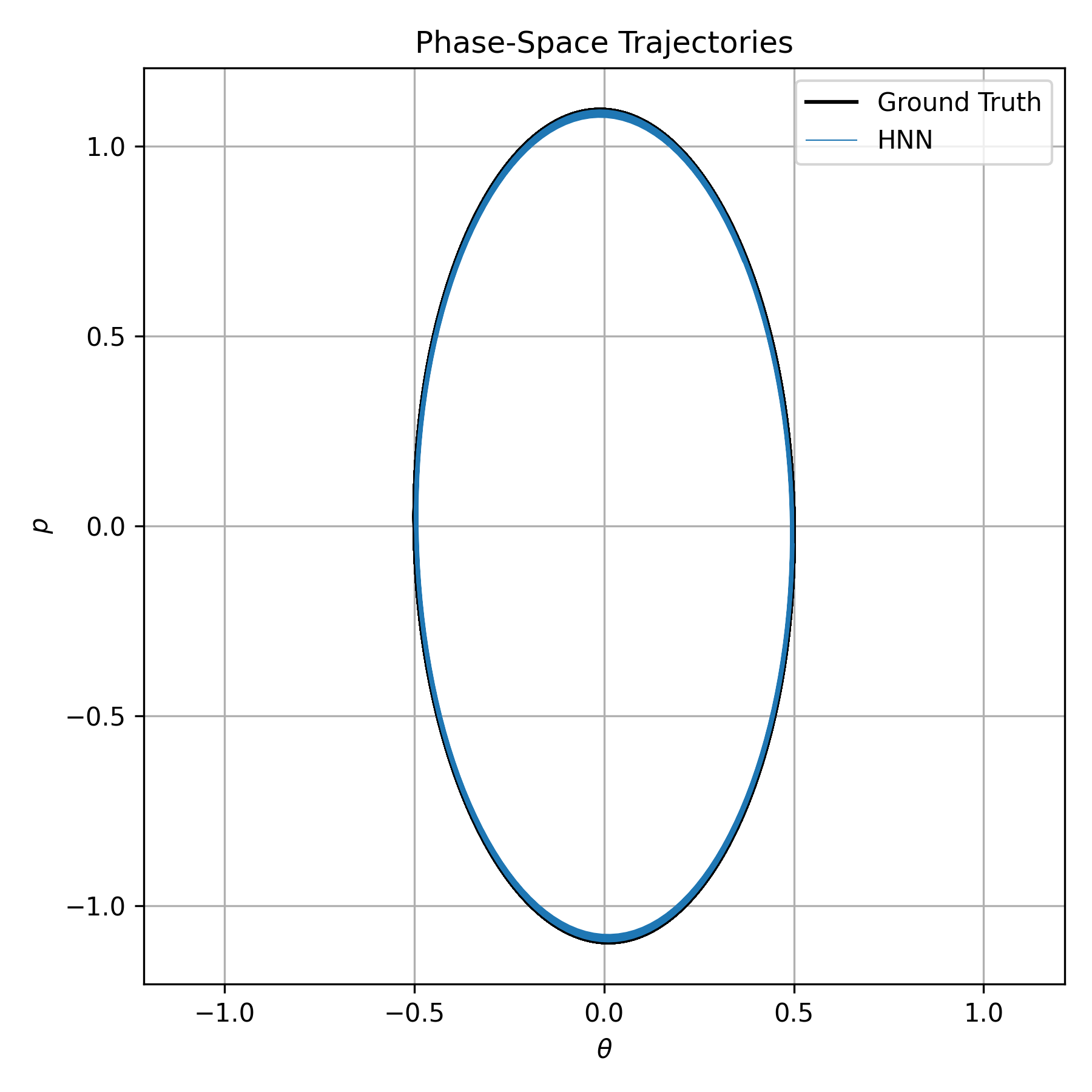
Notice how the network much more closely follows the ellipse, since it implicitly satisfies energy conservation. In the paper, they demonstrate this same idea for more complex physical systems, but I think it’s pretty awesome to see that by enforcing simple physical priors, we can train networks that can better simulate physical systems.